
Heikin-Ashi – An Empirical Study with Ablation, Across Equities, FX and Crypto
Abstract
Heikin-Ashi (HA) candles are a smoothed price representation widely used to read
trend direction. This study asks a precise question: applied mechanically, does
the HA signal carry a risk-adjusted edge beyond an equivalent moving-average
trend rule, and under what conditions? To answer it, the strategy is decomposed
by ablation — HA is removed, the higher-timeframe filter is removed, and the
raw HA signal is isolated — and each variant is run with identical parameters
across 25 equities, 12 FX pairs and 8 crypto assets (2021–2026), with a separate
20-year daily cross-section (2006–2026, 22 names) for robustness. The central
finding is that the HA signal’s marginal contribution is asset-class
dependent: on equities it is negligible (replacing HA with an EMA-cross leaves
median Sharpe essentially unchanged, 0.24 vs 0.21), while on liquid crypto it is
positive (median Sharpe 0.51 vs 0.34; concentrated in BTC and ETH, though the
eight-coin sample is too small and correlated to call a general edge). As a whole, the
composite behaves as a defensive overlay: over 2006–2026 it underperforms
buy-and-hold in return (median +104% vs +937%) but roughly halves drawdown
(−39% vs −63%) and beats buy-and-hold’s cross-sectional median in each of the
three crisis windows tested (GFC, COVID, 2022) by losing less. That protection is
not efficient, however: a passive buy-and-hold de-risked to the strategy’s own
average exposure or volatility delivers the same drawdown at higher return and
better risk-adjusted performance, so most of the drawdown reduction is an exposure
effect rather than skillful timing. Profitability is fragile (transaction-cost-bound
at hourly frequency, median break-even ≈ 0.035% per side among positive-gross
names) and concentrated.
This is exploratory research, not a validated, capital-ready strategy: the
limitations section is explicit about what is not demonstrated. All
experiments are reproducible with the open-source
wichtelm backtester.
1. Introduction
Heikin-Ashi transforms standard OHLC bars into a smoothed series whose body depends on the current and prior bar, producing long single-colour runs during trends. The practical question is not whether HA looks like a trend filter — it does — but whether, applied mechanically, it adds anything over an equivalent non-HA trend rule. A strategy that bundles HA with moving-average filters and stops cannot answer that question on its own: any edge might come from the filters or the stops rather than from HA. This study is built around isolating that contribution.
We measure against buy-and-hold and report the cross-sectional median (robust to the single-outlier distortion that affects the mean), and treat transaction costs and regime behaviour as first-class results rather than footnotes.
2. Data
| Property | Value |
|---|---|
| Intraday set | 25 equities, 12 FX pairs (the 7 majors — EUR/USD, USD/JPY, GBP/USD, AUD/USD, USD/CAD, USD/CHF, NZD/USD — plus 5 high-turnover crosses: EUR/GBP, EUR/JPY, GBP/JPY, EUR/CHF, AUD/JPY), 8 crypto; 1-hour primary, 1-week filter; 2021-01-01 → 2026-06-04 |
| Long-history set | 22 equities; daily primary, 1-week filter; 2006-06-01 → 2026-06-04 |
| Point-in-time membership set (survivorship-bias-mitigated) | 124 names sampled from S&P 500 point-in-time membership (48 delisted/removed in-window); daily primary, 1-week filter; 2006-06-01 → 2026-06-04 |
| Regimes covered | 2021 bull, 2022 bear, 2023–26 recovery (intraday); GFC 2007–09, COVID 2020, 2022 (daily) |
Data hygiene steps that materially affect intraday work:
- Corporate actions. Intraday feeds are raw (not split/dividend adjusted). Several equities split inside the window (10:1, 20:1, 3:1); each was detected as an integer overnight price ratio and back-adjusted. The daily long-history set uses split-and-dividend-adjusted close (an approximate total-return series).
- Bar-grid hygiene. Intraday series can carry duplicate or sub-timeframe timestamps (e.g. around daylight-saving transitions); these were de-duplicated to a strictly increasing grid.
A limitation to state up front: the intraday buy-and-hold benchmark uses raw (price-return) close, while the daily benchmark uses adjusted (≈ total-return) close. Dividends are not credited to the strategy during long periods, nor charged on shorts.
Inclusion criteria. The intraday equity and crypto sets are fixed selections of large, liquid, currently-traded names with full 2021-onward intraday history on the provider — chosen before any results were seen, but currently-listed and hence survivorship-biased (Limitations). The FX set is the seven majors plus the five highest-turnover crosses (§2 table). The 20-year daily set (§4.2) is 22 currently-listed large caps with continuous 2006-onward adjusted history; only the point-in-time membership set (§4.2.1) applies a programmatic, pre-registered inclusion rule — a deterministic 150-name draw from S&P 500 point-in-time membership, with the data-quality and minimum-history exclusions enumerated there.
3. Method
3.1 Strategy and ablation variants
The base (“Full”) strategy is a long-only HA trend rule with a higher-timeframe
filter and a fixed protective stop/target, expressed in the wichtelm DSL:
Feature: HA Strong-Candle Long-Only, 1h primary with 1w trend confirmation
  Primary timeframe: 1h
  Parameter trend_period default 50
  Parameter htf_period default 20
  Parameter stop_loss_pct default 8
  Parameter take_profit_pct default 25

  Background:
    Given a series htf_trend defined as ema(htf_period) on 1w

  Scenario: Enter long on a strong bullish HA candle, intraday and weekly aligned
    Given no open position
    When ha_strong_bullish()
    And price_above_ema(trend_period)
    And close is above htf_trend
    Then long_entry
    And with stop_loss at entry_price * (1 - stop_loss_pct / 100)
    And with take_profit at entry_price * (1 + take_profit_pct / 100)

  Scenario: Exit long on a strong bearish HA candle
    Given a long position is open
    When ha_strong_bearish()
    Then long_exit
To isolate the HA contribution, four variants are tested with identical parameters:
| Variant | HA signal | EMA(1h) | EMA(1w) filter | Stop/target |
|---|---|---|---|---|
| Full | ✓ | ✓ | ✓ | ✓ |
| No-HA (EMA-cross entry/exit) | — | ✓ | ✓ | ✓ |
| No-1w (drop the weekly filter) | ✓ | ✓ | — | ✓ |
| HA-only (raw signal) | ✓ | — | — | — |
The “No-HA” variant replaces the HA entry/exit with a price-vs-EMA cross, holding the filters and stops constant — the direct test of whether HA adds anything. A long/short variant (regime-switched: short only when the weekly trend confirms a downtrend) is tested on crypto, with its own No-HA counterpart.
A precision note on terminology: this design mixes a true ablation with a replacement benchmark. Dropping the weekly filter (No-1w) and stripping the scaffolding (HA-only) are direct ablations — the same signal with a component removed. No-HA is a replacement benchmark: swapping HA entry/exit for an EMA-cross changes the signal’s frequency, latency and holding distribution, so it tests whether HA outperforms a conventional trend signal rather than isolating a single identical signal transformation. That is the right test for the question asked (“does HA beat an equivalent trend rule?”), but it is not a one-variable ablation, and the No-HA comparisons should be read in that light.
3.2 Execution model
Precise execution rules (enforced by the backtester):
- Signal timing. Conditions are evaluated on the close of each primary bar. HA candles are used only to generate the signal (HA primitives resolve against a Heikin-Ashi series); orders execute against the real OHLC series, never against synthetic HA prices.
- Entry fill. A scenario-driven entry fills at the next bar’s open (the signal bar is not itself an executable fill), removing same-bar look-ahead.
- Protective exits.
stop_loss/take_profitare snapshotted at the entry fill and monitored intrabar. The fill is gap-aware: when the level lies inside the bar’s range it fills at the level, but when the bar opens already beyond the level (a gap-through) it fills at the open — the realistic, worse price — not at a level the bar never traded. When both the stop and the target fall inside the same bar’s range, the stop wins (pessimistic convention). - Higher-timeframe filter. The weekly series resolves to the most recently closed weekly bar at each hourly bar — no peeking at an unclosed candle.
- Drawdown is computed mark-to-market on the per-bar equity curve (peak-to-trough), not only on closed trades.
3.3 Metrics
The Sharpe ratio is computed from per-bar returns of the equity curve as
(mean / population standard deviation) × √(periods per year) — i.e. annualised,
with a risk-free rate of zero (it is a raw Sharpe on total returns, not
excess returns) and no autocorrelation correction (Lo, 2002). Two
consequences worth stating: a strategy frequently in cash is not credited a
cash return, and a trend-following return stream’s serial correlation can bias
the annualised figure. Maximum drawdown is the largest peak-to-trough decline of
the per-bar equity curve.
3.4 Experimental design and parameter provenance
The rule is applied with one fixed parameter set (trend_period=50,
htf_period=20, stop=8%, take=25%) to every instrument; these were fixed at
the outset and not optimised per instrument or selected from a sweep, which
keeps the test a measurement of the general signal rather than a fitted result.
Summary statistics are cross-sectional medians. Strategies are compared on
Sharpe and maximum drawdown against each instrument’s own buy-and-hold.
Transaction-cost sensitivity is evaluated across a per-side fee grid and
summarised by the break-even cost. The window spans bull, bear and recovery
regimes, reported separately in §4.3.
3.5 Reproducibility / tooling
All runs use wichtelm: strategies
are plain-text .strat files (the DSL above), runs are TOML, and each emits a
self-contained HTML report (ten risk metrics, equity/drawdown curves, per-trade
breakdown over HA candles). A [sweep] table plus wichtelm sweep runs a
parameter grid ranked by Sharpe, but — per §3.4 — was not used to choose the
reported parameters. The tool does not model commissions or slippage; costs are
applied post-hoc from each run’s round-trip count, keeping the assumption
explicit. Position sizing is a fixed fraction of equity (volatility-scaled sizing
and multi-instrument portfolio construction are out of the tool’s v1 scope — see
Limitations).
4. Results
All figures are gross of costs unless stated.
4.1 Ablation — the Heikin-Ashi contribution
Equities (25, long-only, 1h + 1w, identical parameters):
| Variant | Median return | Median max DD | Median Sharpe | Sharpe > 1 |
|---|---|---|---|---|
| Full (HA+EMA1h+EMA1w+stop) | +3% | −24% | 0.24 | 7/25 |
| No-HA (EMA-cross+EMA1w+stop) | +2% | −26% | 0.21 | 9/25 |
| No-1w (HA+EMA1h+stop) | +18% | −26% | 0.70 | 11/25 |
| HA-only (raw signal) | +18% | −28% | 0.62 | 9/25 |
Two results stand out. First, Full ≈ No-HA (Sharpe 0.24 vs 0.21, drawdown −24% vs −26%): replacing the HA signal with a plain EMA-cross leaves performance essentially unchanged, so on equities HA adds no measurable edge over an equivalent trend rule. Second, in this equity sample the weekly filter behaved as a drag rather than a shield: removing it (No-1w) raises median Sharpe from 0.24 to 0.70 and return from +3% to +18%, for a near-identical drawdown — the filter was sacrificing return for a marginal drawdown change. (Without paired tests or confidence intervals this is a description of the sample, not a generalisation beyond it.)
Crypto (8, long/short, 1h + 1w):
| Variant | Median return | Median max DD | Median Sharpe |
|---|---|---|---|
| Full L/S (HA) | +84% | −67% | 0.51 |
| No-HA L/S (EMA-cross) | +19% | −67% | 0.34 |
Here HA does appear to contribute in this sample: median Sharpe 0.51 vs 0.34, and most visibly on the two most liquid coins — BTC (+329% / Sharpe 1.11 with HA vs +106% / 0.63 without) and ETH (+166% / 0.71 vs +44% / 0.40). The effect is heterogeneous (on SOL the EMA version still wins outright). With only eight correlated, ex-post-selected and survivorship-biased instruments, this is not enough to establish a general crypto edge: the defensible statement is that in this small crypto sample the HA variant produced a higher median risk-adjusted result, concentrated in BTC and ETH. Confirming a real edge would need paired instrument-by-instrument tests, bootstrap confidence intervals, an out-of-sample window, and a point-in-time crypto universe with realistic short funding.
4.2 Long-history robustness (daily, 2006–2026)
Over a 20-year daily cross-section (22 names, identical rule):
| Window | Median return | Median max DD | Median Sharpe | Beats B&H | B&H return | B&H max DD |
|---|---|---|---|---|---|---|
| Full 2006–2026 | +104% | −39% | 0.30 | 0/22 | +937% | −63% |
| GFC 2007–2009 | −5% | −20% | −0.12 | 14/22 | −16% | −59% |
| COVID 2020 | −2% | −7% | −0.16 | 13/22 | −2% | −36% |
| Bear 2022 | +2% | −12% | 0.27 | 15/22 | −9% | −30% |
Over the full 20 years the strategy underperforms buy-and-hold by a wide margin (+104% vs +937%, beating it on 0 of 22 names) while roughly halving the drawdown (−39% vs −63%). Its relative strength is concentrated in crises: in the GFC, COVID and 2022 it beat buy-and-hold on a majority of names by losing less. This is the defining profile of a defensive trend overlay across multiple independent regimes.
The §4.2 cross-section uses 22 fixed, currently-listed names, which is survivorship-biased (it cannot see companies that left the index or went to zero). The next subsection materially mitigates that bias by including point-in-time membership and delisted constituents.
4.2.1 Point-in-time membership aggregate (survivorship-bias-mitigated, daily, 2006–2026)
To mitigate survivorship bias and to report an actual portfolio (not a median across independent runs), the strategy was re-run over a point-in-time S&P 500 membership sample: a deterministic 150-name sample drawn from the index’s point-in-time historical membership (every name that was a constituent at any time in the window, including those later delisted or acquired), with each name backtested only over its membership interval. After excluding 13 names for data-quality breaks (see below) and 13 with insufficient history, 124 names remained, of which 48 were delisted/removed during the window — i.e. failed companies are included, not silently dropped. The aggregate is an equal-weight buy-and-hold portfolio ($1 per name at entry, held; a delisted name’s capital is banked at its terminal value), compared against the same strategy:
| Series | Total return | Max drawdown | Sharpe |
|---|---|---|---|
| Buy & hold (equal-weight) | +582% | −51% | 0.62 |
| Strategy (gross) | +53% | −19% | 0.39 |
| Strategy (net @0.02%/side) | +45% | −20% | 0.35 |
| Strategy (net @0.05%/side) | +35% | −20% | 0.29 |
Robust median per name (no aggregation choice): strategy +6% vs buy-and-hold +100%; the strategy beat buy-and-hold on 31 of 124 names (25%).
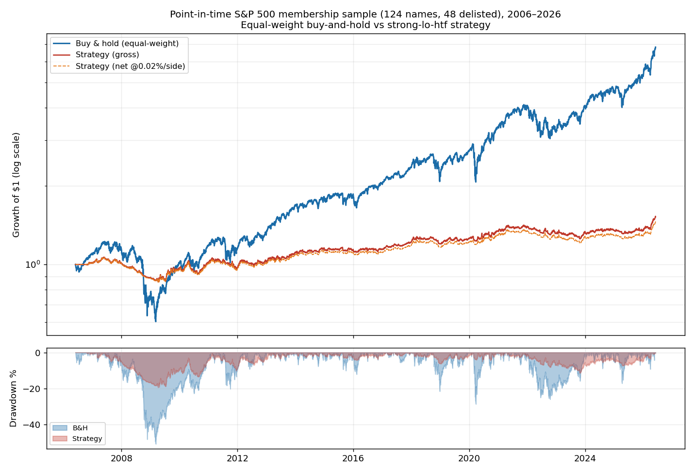
The point-in-time-membership result confirms and sharpens §4.2: buy-and-hold returns roughly eleven times as much (+582% vs +53% gross), and the strategy’s only durable advantage is drawdown — it more than halves the worst peak-to-trough decline (−19% vs −51%), visible in the underwater panel during 2008, 2020 and
- On a risk-adjusted basis buy-and-hold still wins (Sharpe 0.62 vs 0.39). Because the rule is low-turnover at the daily frequency, the tested explicit fees move the result only modestly (+53% → +45%). The economic reading is unchanged across the survivorship-biased and survivorship-bias-mitigated cross-sections: this is a defensive overlay that trades the large majority of compounding for a smoother ride.
A data-quality caveat that also bears on methodology. The price series were pulled by bare ticker from a single price-only provider, which reuses delisted symbols for unrelated (often penny-stock) entities and occasionally serves unadjusted corporate actions. This produced impossible single-day moves for former S&P 500 members (e.g. the tickers once belonging to Pepsi Bottling Group, Heinz and Merrill Lynch), which were detected as >+80%/−60% daily jumps and excluded (13 of 137 names with data, concentrated in delisted tickers). A publication-grade survivorship-free study needs a provider with point-in-time ticker-to-entity mapping (e.g. CRSP, Norgate, Sharadar); the exclusion here is a declared data hygiene step, not a performance filter, and one delisted name (Lehman Brothers) had no usable series at all. Because the exclusions concentrate in delisted tickers, this set is best described as survivorship-bias-mitigated, not bias-free; a natural robustness check (left as future work) is to re-bank each excluded name’s terminal capital under optimistic / −50% / zero scenarios and confirm the conclusions are unchanged.
4.2.2 Is the drawdown reduction protection, or just less exposure?
The “defensive overlay” reading is descriptively true but does not, on its own, show the strategy provides efficient protection: any rule that sits in cash much of the time mechanically cuts return, volatility and drawdown. The honest test is to neutralise the exposure and compare against passive benchmarks built to the same risk. The strategy is invested only about 27% of the time (median per-name time-in-market 30%; its realised volatility is ≈ 0.32× the index’s). Two exposure-neutral benchmarks on the point-in-time membership portfolio:
| Series | Total return | Max drawdown | Sharpe | Calmar |
|---|---|---|---|---|
| Buy & hold (100% invested) | +582% | −51% | 0.62 | 0.20 |
| Strategy (gross) | +53% | −19% | 0.39 | 0.11 |
| Exposure-matched B&H (static 27% index / 73% cash) | +79% | −16% | 0.62 | 0.18 |
| Volatility-matched B&H (index scaled ×0.32) | +100% | −19% | 0.62 | 0.19 |
Both passive benchmarks are built from the same equal-weight point-in-time membership portfolio used in §4.2.1. Their daily portfolio returns are multiplied either by the strategy’s time-weighted average gross exposure (0.27) or by the ratio of strategy-to-benchmark realised volatility (0.32, on coincident daily returns), with the residual allocation earning a flat 0% and with no leverage or rebalancing costs; Sharpe and Calmar are computed by the same method as for the strategy. Both passive benchmarks dominate the strategy. A static “27% index, 73% cash” mix — the strategy’s own average exposure, with no timing whatsoever — earns more (+79% vs +53%) at a smaller drawdown (−16% vs −19%) and higher risk-adjusted return (Sharpe 0.62 vs 0.39, Calmar 0.18 vs 0.11). Scaling the index to the strategy’s volatility tells the same story (+100% vs +53% at identical drawdown). In other words, on this 20-year cross-section the strategy’s market-timing subtracts value relative to naively holding less of the index: the drawdown reduction is an exposure effect, not evidence of skillful protection. (Cash is credited a 0% return here, matching the strategy’s own convention. Crediting a positive cash rate would improve both the strategy and the de-risked passive benchmarks — both sit ≈73% in cash on average — and its effect on their relative ranking has not been modelled.)
4.3 Regime sub-periods (intraday, 2021–2026)
| Equities long-only | Median return | Median max DD | Median Sharpe |
|---|---|---|---|
| 2021 bull | −0% | −11% | 0.06 |
| 2022 bear | −2% | −12% | −0.35 |
| 2023–26 recovery | +9% | −14% | 0.79 |
On equities the long-only rule reduced drawdown in the 2022 bear (−12% vs a much deeper buy-and-hold decline) but did not profit there (Sharpe −0.35); its gains accrued in the recovery. So “protection” here means smaller losses, not positive returns.
| Crypto long/short | Median return | Median max DD | Median Sharpe |
|---|---|---|---|
| 2021 bull | −4% | −42% | 0.16 |
| 2022 bear | +20% | −37% | 0.65 |
| 2023–26 recovery | +32% | −52% | 0.48 |
On crypto the long/short rule profited in the 2022 bear (+20%, Sharpe 0.65) via the short side — the regime where the short leg earns its keep.
4.4 Timeframe granularity (a preliminary probe)
Moving the composite’s primary timeframe from daily to hourly (weekly filter
fixed) raised median Sharpe 0.32 → 0.87 and cut drawdown −20% → −13% on a
four-instrument probe. This is not a clean isolation of timeframe, and
should be read only as preliminary: holding EMA(50) and the 8%/25% stops fixed
means the hourly run also has a far shorter economic lookback (≈ 50 hours vs
≈ 50 days) and different effective stop distances, so the signal’s horizon changes
along with the bar size. An isolated test would hold the lookback in market time
constant (≈ 50 daily bars vs the equivalent count of hourly bars). With only four
instruments and that confound, no weight should be put on the magnitude; §4.1
separately shows the HA component is not what drives the composite on equities.
4.5 Cross-sectional heterogeneity (a hypothesis, not a result)
The 25-equity cross-section is bimodal: seven names show Sharpe > 1 while the rest cluster near zero. This cluster is identified ex post — using the very outcome it would explain — so it cannot be read as evidence that “the edge is real.” It generates a testable hypothesis: that ex-ante trend persistence (measured on a prior window, without using strategy returns) might identify more suitable instruments. Validating that requires an out-of-sample test and is left as future work; the backtest-overfitting literature (Bailey et al.) shows how quickly ex-post subgroup selection manufactures apparent edge.
4.6 Transaction-cost break-even
An hourly rule executes 300–900 round trips over the window. Under a
multiplicative cost model (net ≈ gross × (1 − 2f)^N), net return is highly
fee-sensitive. Among the equities with positive gross return, the median
break-even cost was ≈ 0.035% per side — i.e. half of that positive-gross
subset (not half of all 25) lose their edge at any realistic retail commission.
The (1 − 2f)^N factor is a deliberately pessimistic approximation of the exact
proportional-fee adjustment (1 − f)^(2N) (two executions per round trip): it
drops the +f² per round trip, so it slightly overstates the cost at the fee
levels tested. The model also charges a flat fee per round trip rather than per
traded notional; this matches notional to equity only because every run is sized
at 100% of equity (notional ≈ equity each fill), and would need to be applied
to each fill’s actual notional under fractional or volatility-scaled sizing. It
also omits bid-ask spread, slippage, market impact, borrow/funding costs on
shorts, and dividend obligations; the real cost hurdle is therefore higher than
the headline figure.
4.7 The short side is asset-class dependent
Adding a regime-switched short side helps crypto (§4.1, §4.3) but degrades equities (median Sharpe falls, drawdown rises) and range-bound FX (more trades, worse net). On the 12-pair FX cross-section the short side roughly doubles the trade count (e.g. EUR/USD 382 → 922 round trips over the window) and pushes the median FX result from marginal to negative (median FX Sharpe −0.17 long-only → −0.15 long/short, median net-of-cost return −16% → −30%); only the JPY pairs with a genuine 2021–2024 USD-trend (USD/JPY) carry a positive gross Sharpe, and even those are cost-bound. Shorting individual equities works against the equity risk premium and is whipsawed by bear-market rallies; FX 2021–2026 offered little sustained trend either way; crypto, lacking a structural upward drift and exhibiting long two-way trends, is where the short side adds value. (Borrow cost and short-squeeze risk on equities are not modelled, so the real short-side equity result is worse than shown.)
The FX set was widened from the original eight to all seven majors plus five high-turnover crosses (adding NZD/USD, GBP/JPY, EUR/CHF and AUD/JPY) to confirm the result is not an artefact of pair selection — it is not; the broadened cross-section tells the same story. One honest data caveat: EODHD’s NZD/USD intraday history is much shorter than the other pairs (≈ 8.6k 1-hour bars vs ≈ 27.7k), so its backtest spans a narrower effective window and its lone bright spot (a long-only Sharpe above 1 on only ~140 trades) rests on thin data and should not be over-read.
4.8 ATR-based stops — a note
Replacing the fixed-percentage stop/target with an ATR-distance (chandelier) stop was attempted as a robustness check. On equities it is straightforward; on volatile crypto long/short it became pathological — a tight ATR stop in a high-volatility regime is hit and re-entered constantly, producing an extreme trade count (and, mechanically, prohibitive transaction costs).
| Variant | Median return | Median max DD | Median Sharpe |
|---|---|---|---|
| Equities long-only — ATR-stop (3×ATR / 6×ATR) | +5% | −24% | 0.31 |
| Equities long-only — fixed % (8/25, ref) | +3% | −24% | 0.24 |
| Crypto long/short — ATR-stop (3×ATR / 6×ATR) | +48% | −66% | 0.41 |
| Crypto long/short — fixed % (8/25, ref) | +85% | −67% | 0.52 |
On equities the ATR stop is a mild risk-adjusted improvement (median Sharpe 0.24 → 0.31) at the same drawdown (−24%); on crypto long/short it lowers the median Sharpe (0.52 → 0.41) for no drawdown benefit — the trade-count degeneracy showing through in the medians. That degeneracy is itself the point: a volatility-scaled stop alone, without a corresponding volatility-scaled position size, does not give a clean cross-asset comparison — it simply trades more where volatility is higher. The normalisation the cross-asset comparison actually needs is volatility-scaled sizing (constant risk per trade / portfolio vol target), which is out of the backtester’s scope (Limitations) and is the right subject for a dedicated follow-up.
5. Discussion
The ablation reframes the headline. The drawdown reduction and the defensive profile come from the trend-rule-plus-stop composite, not from Heikin-Ashi specifically: on equities a plain EMA-cross matches HA, and the weekly filter actually subtracts. And the drawdown reduction itself is largely an exposure effect — a passive buy-and-hold de-risked to the same exposure or volatility beats the strategy (§4.2.2). The only place HA shows a positive marginal contribution is the small, correlated crypto sample (concentrated in BTC and ETH), where eight survivorship-biased instruments are too few to call it a general edge. The most defensible one-line summary is therefore:
A multi-filter trend-following composite can reduce drawdown and lose less than buy-and-hold in crises, but the drawdown reduction is largely an exposure effect a de-risked buy-and-hold reproduces, its profitability is fragile, concentrated and cost-dependent, and the Heikin-Ashi component shows a positive contribution only in a small liquid-crypto sample — not on equities.
This is consistent across a 20-year daily sample and three intraday regimes, so the observed profile is not confined to a single selected market episode within this dataset — but, with selected windows, in-sample tests and no out-of-sample validation, it is specific to this rule set, parameters, cost environment and instrument universe.
6. Limitations (what this study does not establish)
- It does not prove an HA edge in general. §4.1 shows HA’s equity contribution is ≈ 0 over an EMA-equivalent; the title is about the composite, with HA isolated.
- No volatility-scaled position sizing. Out of the backtester’s v1 scope; sizing is a fixed equity fraction, so cross-asset comparisons mix signal, volatility and sizing.
- Aggregate portfolio only for the point-in-time membership daily set. §4.2.1 reports an equal-weight buy-and-hold aggregate; every other cross-section is a median across independent runs, which is not a directly investable portfolio. Correlated instruments (8 crypto, USD-sharing FX) are not independent observations.
- Survivorship bias only mitigated, and only for the large-cap daily set. §4.2.1 uses point-in-time S&P 500 membership including delisted names; the intraday 25-equity, FX and crypto sets still use a fixed, currently-traded selection and remain survivorship-biased. The membership set also required a declared data-hygiene exclusion (13 of 137 names) for ticker-reuse breaks from a price-only provider, concentrated in delisted tickers — so it is survivorship-bias-mitigated, not bias-free; point-in-time ticker-to-entity mapping (CRSP, Norgate, Sharadar) is needed for a fully clean run.
- Costs are modelled post-hoc and omit spread/slippage/impact/borrow/funding; the break-even is computed on the positive-gross subset.
- No out-of-sample / walk-forward validation and no deflated Sharpe. A single in-sample window is used; the ex-post cluster (§4.5) is a hypothesis.
- Benchmark asymmetry. Intraday B&H is price-return; daily B&H is adjusted (≈ total-return); dividends are not credited to the strategy or charged on shorts.
- Sharpe uses a zero risk-free rate and no autocorrelation correction (§3.3).
7. Conclusion
Treated as a mechanical system and tested honestly — with the Heikin-Ashi signal ablated out, across asset classes, over a full 20-year cross-section and three intraday regimes — Heikin-Ashi trend-following is best understood as a defensive overlay: it gives up most of a rising market’s return but roughly halves drawdown and loses less than buy-and-hold in crises. This profile remains visible once survivorship bias is mitigated — on a point-in-time S&P 500 membership sample that includes delisted names, buy-and-hold compounds roughly eleven times as much while the strategy more than halves the drawdown (§4.2.1) — though ticker reuse, missing histories and the data exclusions stop short of a fully survivorship-free estimate. But the protection is not efficient: a passive buy-and-hold de-risked to the strategy’s own exposure or volatility delivers the same drawdown at higher return and a better Sharpe and Calmar (§4.2.2), so the drawdown reduction is largely an exposure effect rather than skillful timing. Its profitability is fragile and cost-bound at high frequency, and its specific Heikin-Ashi ingredient shows a positive contribution only in a small liquid-crypto sample (BTC, ETH) too limited to call a general edge — not on equities, where an equivalent moving-average rule performs the same. The result is solid exploratory research and a set of testable hypotheses — not a validated, capital-ready strategy.
Reproducibility & disclaimer
The backtester, strategy DSL and configurations are open source at
wichtelm-app. Price data was
snapshotted from a commercial provider and split-adjusted (equities); the
licensed price series is not redistributed. The S&P 500 point-in-time membership
(§4.2.1) is from the public
fja05680/sp500 dataset; the equity curves
shown are derived performance indices (growth of $1), not raw prices, so they
contain no redistributable licensed data. Transaction costs were applied post-hoc
from each run’s round-trip count. For reproducibility the runs are pinned to a
fixed build: every result here was re-run end-to-end on wichtelm-app commit
6ee5a1c (the gap-aware protective-fill build, merged to main via PR #64) and
reproduced to the
reported precision; the FX cross-section was additionally broadened from eight to
twelve pairs (§4.7). The strategy .strat files are reproduced verbatim in §3.1
and §3.4 fixes the one parameter set used throughout; the per-run TOML configs and
the licensed price snapshots are not redistributed.
This article is for research and educational purposes only. It is not financial advice. Past performance is not indicative of future results, and hypothetical backtested results carry well-documented biases.